Assistance with MS365 - Excel (its up to date) and Conditional Formatting

[ladyck3]

Assistance with MS365 - Excel (its up to date) and Conditional Formatting

I have no clue how to use this tool anymore, ever since the update. I sure hope this is the right way to go about this. A few things you should about my capabilities.
I have been retired over a decade and if you don't use it, you do certainly lose it. In this case, if you were to provide an answer using VBA, please don't. I do not now,
nor have I ever understood it and I am so flustered right now that trying to teach this old dog "you just gotta do this or that" will fall on deaf ears. Steps, please...

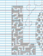
The information attached is just a small part of the chart I am working on and have not included the entire workbook as it is copyrighted material. I am attempting to make changes to this data for myself and no one else. This is a crochet pattern and its worked from lower right to left and work up the chart from the bottom to the top. This segment has simply a capital "L".

Being left handed, I have cell number both right to left and left to right and the rows on once side even number, and the other the odd number rows.
I work left to right and upward....

So this is what I am attempting to do and that is, as you can see on the left, ever other row is either light blue or lavender. HOWEVER, the grey cells (the pattern stitches) are in grey. I need to change each row color to correspond with either the blue or lavender on all blank/white cells but the grey cells should remain untouched. I will place strategic "X's" in the appropriate spots to designate the type of stitch to use. I just need the colors of the white cells, per row, to change.

I figure conditional formatting? But I have absolutely NO BLOODY IDEA how to even start to play with a formula. Can you help??? PLEASE. And again, I was retired with tek-tips changed and have not really been using thie resource like I did when working so I hope that I am in the right category or location and I hope that I posted the inquiry properly. HELP! Seriously... I'm too flustered and frustrated to go on with this project without the kind help from y'all. SKIP you still around? Again, I just don't get VBA so if you write me code to F-whatever and enter it some place it does me no good because I don't know how to adjust or edit it. Can this be done via Conditional Formatting? OR... do I just abandon this project. I've had the pattern for 4 years, really REALLY want to make it but as is, its not written for "Mosaic" crochet, its meant for "Interlock" crochet only. I know, out of your realm but thus is my issue.

Most sincerely,
Laurie K.

 

[Jim E]

Can you simplify? As an example, do you want the background fill changed based on the value of a cell?

if A1 = A, change the color to red
If A1 = B, change the color to green
If A1 = blank, change the color to gray.

It sounds like this can be done by conditional formatting, with no VBA needed. Let us know!

 

[ladyck3]

Hi Jim,

Thanks for getting back to me. The numbers you see have NOTHING to do with any value to be concerned over. These are line numbers on left & right by 2x's, left the even rows 50, 48, 46, on the right the odd numbers.... 49, 47, 45. They should not be consideration of any conditional formatting.

I honestly don't understand the A1 references you mention, sorry.

It really, in theory seems simple, Im just not a conditional Formatting guru.

I will add X marks manually in the grey areas where shown...as needed. However to help make sense of where they belong are dependent as to whether they are on either a light blue row (color 1) or on a lavender row (color 2). I NEED the Grey to remain grey. All of the white/empty squares should be light blue or lavender every other line. All even number rows, light blue, all odd number rows lavender, or vice versa.

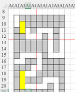
The ENTIRE chart is 150 columns across (width) and 150 rows in length. The sample is just a snippet. Those columns in yellow are just there (not to be touch) but rather, I guess you could call them anchor markings to help keep track of where you are while stitching.

Does this. At all clear some of this up? Im doing this from phone...sorry for any typos.

Laurie

 

[Jim E]

Hi, If you are uploading a sample file, I'm not seeing it.

A1, A2, etc. are cell references. If you are manually typing in a specific value in a cell, a conditional format will change it to whatever color you specify for that value, but it not based on the row or column.

So if you manually type in the letter B in a cell, you can have that cell or any other change color.
If you want every other row to be a different color, you can use Excel's banding option. Here's how:

• Select the block of cells.
• Go to the Home tab.
• Click Format as Table in the Styles group.
• Choose a style with banded rows.
• Confirm the range and whether your table has headers. You can also click on/off the other options to see the results.
• Done! The banded colors apply automatically.

Try this, maybe I'll get one right if I understand what your looking to do!

Regards

 

[Andrzejek]

Since we cannot see your example, we are going to play a guessing game.

You said:
" I need to change each row color to correspond with either the blue or lavender on all blank/white cells but the grey cells should remain untouched. [...] I just need the colors of the white cells, per row, to change."

my guess would be: you can Filter -- Filter by Color... and have your sheet show which Rows are displayed based on the color. So if you select 'No Fill' that will Filter your Rows and show only "blank/white" rows,

Just a guess here....

 

[Jim E]

Hi,

The A1, A2 are cell references in Excel's naming convention.
Excel sequentially labels all (width) columns in a worksheet starting with A, B, C, ... X, Y, Z, AA, AB.
Similarly, Excel sequentially numbers (height) all rows starting with 1, 2, 3 ...

As an example, cell A2 has a value of X.

A B C D E
1
2 X
3
4
5

Does this help? Conditional Formatting can be programmed to turn cell A2, or any other cell, any color you want. No value (or spaces) in A2 would leave the target cell's color unchanged. Since you said you would manually put an X in a cell, this could work for you.
As an example, if cell A2 had a value of X, conditional formatting could change cell E2 background color to blue, while the value in cell E2 remained unchanged.

Also, you mentioned the size of the work area, 150 by 150. If you highlight this block of cells with your cursor (the area will turn a shade of gray), you can use the steps in the previous message to turn every other row a different color, either from the options given or your own choices.

Regards

 

[ladyck3]

Since we cannot see your example, we are going to play a guessing game.

You said:
" I need to change each row color to correspond with either the blue or lavender on all blank/white cells but the grey cells should remain untouched. [...] I just need the colors of the white cells, per row, to change."

my guess would be: you can Filter -- Filter by Color... and have your sheet show which Rows are displayed based on the color. So if you select 'No Fill' that will Filter your Rows and show only "blank/white" rows,

Just a guess here....

Oh Andy... umm HUH? LOL

Hi, If you are uploading a sample file, I'm not seeing it.

A1, A2, etc. are cell references. If you are manually typing in a specific value in a cell, a conditional format will change it to whatever color you specify for that value, but it not based on the row or column.

So if you manually type in the letter B in a cell, you can have that cell or any other change color.
If you want every other row to be a different color, you can use Excel's banding option. Here's how:

• Select the block of cells.
• Go to the Home tab.
• Click Format as Table in the Styles group.
• Choose a style with banded rows.
• Confirm the range and whether your table has headers. You can also click on/off the other options to see the results.
• Done! The banded colors apply automatically.

Try this, maybe I'll get one right if I understand what your looking to do!

Regards

Jim, I thought about this and then it hit me... this won't color all lines to be all blue and whte or whatever.... there is something in the grey boxes... the color itself. I'm aware of how to insert a table and edit it. I gave it a shot and it did what I'm seeking, the easiest way that I can even comprehend that I should have first throught of on my own. Geeesh, Laurie... get a grip.. LOL Yes, you got this right... it suits the purpose I'm seeking. TA-DA! I'm honored to be your first "one right" ... LOL <old lady sense of humor> hehehehe

 

[ladyck3]

Hi, If you are uploading a sample file, I'm not seeing it.

A1, A2, etc. are cell references. If you are manually typing in a specific value in a cell, a conditional format will change it to whatever color you specify for that value, but it not based on the row or column.

So if you manually type in the letter B in a cell, you can have that cell or any other change color.
If you want every other row to be a different color, you can use Excel's banding option. Here's how:

• Select the block of cells.
• Go to the Home tab.
• Click Format as Table in the Styles group.
• Choose a style with banded rows.
• Confirm the range and whether your table has headers. You can also click on/off the other options to see the results.
• Done! The banded colors apply automatically.

Try this, maybe I'll get one right if I understand what your looking to do!

Regards

See below... it worked! more detals below.

 

[Andrzejek]

Like I said, a guessing game.

It would help a LOT if you would include 2 pictures (worth a 1000 words):
Picture 1 - this is what I have now.
Picture 2 - this is what I would like to have.

Pictures do not have to be big, just enough to show your need.

 

[ladyck3]

Like I said, a guessing game.

It would help a LOT if you would include 2 pictures (worth a 1000 words):
Picture 1 - this is what I have now.
Picture 2 - this is what I would like to have.

Pictures do not have to be big, just enough to show your need.

I did include a clip of the spreadsheet itself on the initial post, Andy.... but its cool. I appreciate it that you jumped in

 

[ladyck3]

Well Andy, I did include a truncated version of the chart, I don't see it now... what happened to it??
OOOOOOOOOOoooooooooooooooo I attached the *.xlsx file (which I see now is not allowed) DUH ME...
so I zipped it up... this, I THOUGHT went with the initial post. <slapping self on wrist> "Dunderhead, Laurie" LOL

 

[Andrzejek]

I assume what you have attached is what you have now to start with. That would be Picture 1
How about Picture 2 - "this is what I would like to have". Doesn't have to be big, just 10x10 cells would do.

I see you have some merged cells - highlighted here is yellow

 

[ladyck3]

I realize that I'm being a big vague, but its on purpose, because this is not a business thing, its for my favorite craft, CROCHET.
I guess the very BEST way to explain it is to have you see the Video (not the specific chart in the video, just a chart without X's that require an "X" where a different stitch is used.)

Having the lines, / white cells / being 'coded' for lack of a better word, to show line colors, as Ashlee shows in Pink and whatever. Interlock does not require "X" for instruction, however Mosaic Overlay (what I"m trying to use) DOES require the "X". So yes, the white squares being white or blue is fine, its imparative that the grey is untouched by another color. The yellow parts you highlight will be ...because I'm using blue/white table/cell shading... is a good thing.

Seriously, it will be a LOT to put in the Xs required because this chart is 150 rows tall by 150 stitches wide and the ENTIRE pattern is all flowers and other entities... it will take longer to mark it up than it will take to make the darn thing... but I'm just that stubborn. LOL

I'm happy with the every other row, because the "Grey" are not over-written with other colors and I can pencil over parts I've stitched to keep my place in progress.

I'm good... honest