Sum in Pivot? 1

[supportsvc]

Please see image

Need to have the QOO, QPO and the Months summed to calculate against the item QOH as a single row

 

[combo]

What excel version do you have?
Could you post sample data that generates the above report (best as workbook or table to copy)? Do you need only one output line or multiple records? In the second case what is the rule of aggregation (maybe at least screenshot od table design)??


combo

 

[SkipVought]

Just to clarify, (as it will help my understanding) I'm making a guess...
QOH - Qty ON HAND
QOO - Qty ?? ON ORDER
QPO - QTY ?? PURCHASE ORDER

Then you have, in effect, at least two implied formulas...
QOO = SUM(MONTHS) ???
Qty Available = QOH - (QOO + QPO) ???

Don't know anything, according to your example, about QPO.

With that stated, when I have had need to display data in a pivot (not necessarily a Pivot Table) that has somewhat complex math required as in your case (still in the dark about QPO) I used Multi-Criteria array math formulae like SUMPRODUCT() to get the desired results.

But FIRST we need clarification about QPO and some valid sample data.

Skip,

_{Just traded in my OLD subtlety...
for a NUance!}

 

[supportsvc]

Sorry,
Yes you are correct on what the acronyms stand for.

The Available column is a formula
QOH - QOO + QPO

I've included the Worksheet with the Pivot

QOO is the sum of the monthly columns, however they want to see 6 months and the average over the 6 month period along with what's available for the ItemCode.

Hope that helps?

 

[SkipVought]

Could you post sample data that generates the above report

The workbook you uploaded, doesn't really help. We need to see your Source Data that you used to make your PT.

Skip,

_{Just traded in my OLD subtlety...
for a NUance!}

 

[supportsvc]

It's linked to a SQL View

The data set is a formulated set that produces the Quantity Ordered from SalesOrder history tables by month for the past 6 months.

The Quantity On Hand and Quantity On Purchase Order comes from the Item by Warehouse table that stores this info.
The QOO is the same as show in the monthly columns but in the Pivot, it creates a separate line for each month's quantity.

Trying to show the sum of the QOO in the QOO column, which should be the total of the 6 months vs. showing it each time there's Quantity sold in each month.

The example shown and the worksheet with the entire Pivot shows the data and what they represent in regards to the
QOH
QOO <-- and how this is dervied
QPO

 

[SkipVought]

Okay. I tried to simulate your source table, tDTA in sheet [highlight #4E9A06]SrtDta[/highlight]
[pre]
ProductType ItemCode ItemCodeDesc QOH QPO Dte Qty
F 100KIFS 100GSM WHITE King Fitted Sheet 150 0 1-May 1
F 100KIFS 100GSM WHITE King Fitted Sheet 150 0 1-Jun 3
F 100QUFS 100GSM WHITE Queen Fitted Shee 155 0 1-Apr 1
F 100QUFS 100GSM WHITE Queen Fitted Shee 155 0 1-Feb 2
F 100QUFS 100GSM WHITE Queen Fitted Shee 155 0 1-May 4
F 100QUFS 100GSM WHITE Queen Fitted Shee 155 0 1-Jun 15
[/pre]

Here's my solution assuming that the source table data for the desired date range has been downloaded to a sheet and that table in Excel I call tDTA, a Structured Table.

My QUERY results is this in sheet [highlight #4E9A06]InvPru[/highlight]...
[pre]
ProductType ItemCode ItemCodeDesc QOH QPO
F 100KIFS 100GSM WHITE King Fitted Sheet 150 0
F 100QUFS 100GSM WHITE Queen Fitted Shee 155 0

[/pre]

Then I added these heading for the pivot...
[pre]
[highlight #FCAF3E]2018[/highlight] 1 2 3 4 5 6 7 8
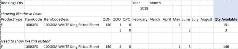
ProductType ItemCode ItemCodeDesc QOH QPO QOO Jan Feb Mar Apr May Jun Jul Aug Qty Available
F 100KIFS 100GSM WHITE King Fitted Sheet 150 0 4 [highlight #FCE94F]0[/highlight] 0 0 0 1 3 0 0 146
F 100QUFS 100GSM WHITE Queen Fitted Shee 155 0 22 0 2 0 1 4 15 0 0 133
[/pre]

The Formula
[tt]
[highlight #FCE94F]=SUMPRODUCT(
(tDTA[Qty])*
(tDTA[ProductType]=[@ProductType])
*(tDTA[ItemCode]=[@ItemCode])
*(tDTA[ItemCodeDesc]=[@ItemCodeDesc])
*(tDTA[QOH]=[@QOH])
*(tDTA[QPO]=[@QPO])
*(tDTA[Dte]=DATE([highlight #FCAF3E]SelectedYR[/highlight],G$1,1)))[/highlight]
[/tt]

I have uploaded your workbook with my additions

Oh, yes, here's my SQL

SELECT DISTINCT
  a.ProductType
, a.ItemCode
, a.ItemCodeDesc
, a.QOH
, a.QPO
FROM `C:\Users\Skip\Downloads\InventoryPurchasing.xlsx`.`SrcDta$` a

Skip,

_{Just traded in my OLD subtlety...
for a NUance!}

 

[supportsvc]

Thank you

That gave me an idea.
I removed the QOO from the source data and added after the last month and before the Qty Available column.
All the columns from QtyAvailable are formulated columns.
Inserted QOO as a formula field and did a sum of the 6 months then updated the QtyAvailable.

Much easier and quicker

 

[SkipVought]

Skip,

_{Just traded in my OLD subtlety...
for a NUance!}